[dsp] Speech Digital Signal Process Review
11 Nov 2019 by BY Zhi-kai Yang
For I have few oppotunities to study DSP(Digital Signal Processing) systematically, I intend to gather some of key knowledge and processing tricks here for the following research.
-
Where do I need DSP method?
Recently I am ongoing the studies of Detecting Depression via a Multi-Media model. I need to process the digital signal like video and sound which need some basic knowlege about Speech Processing and Compuer Vision. And DSP lay the base for them. For I am oriented by practicing, I will introduce the programming tricks firstly, then codes and mathmatics will combine. Only main concepts in DSP of course. This article focus on speech signal first.
-
What I will cover
- Signals, Wave, Spectrum
- Analytics Method (DCT, FFT)
- Spectrum Research (Convolution, Filter, Autocorrelation, Defferentiation and Integration)
- Cepstrum
-
Programming Tools
Though
Matlabis a greet tool for DSP, I will use more light toolScipy.signalandScipy.fftpackinPython.Scipyincludesnumpuy,matplotlib.The majority of the following codes are reffered to ThinkDSP. However, the origin book’s code are highly wrapped so that the author can explain the objects more comprehensively. I try to extract the main idear of the code and display it linearly for a convinient review.
Signals, Wave and Spectrum
First research object includes signals, wave and spectrum.
A signal represents a qunatity that varies in time. Its processes are systhesizing, transforming and analyzing.
A Wave represents a signal evaluated at a sequence of points in time ts (also calledframe), and computing the corresponding values of signals ys.
import numpy as np
PI2 = np.pi * 2
# make a signal
freq = 440
amp = 1.0
offset = 0,
func = np.sin
In fact, the aboved parameters can simulate a sine and cosine wave first like $ys = sin(2\pi ft)$, but it is continous in time. We have to evaluate the signal into Wave form to plot it.
duration = 1
start = 0
framerate = 11025

# transform to wave
n = round(duration * framerate) # total number of frames
ts = start + np.arange(n) / framerate # sampling time point corresponding to each frame
phases = PI2 * freq * ts + offset
ys = amp * func(phases)
Then, we plot the Wave.
%matplotlib inline
import matplotlib.pyplot as plt
plt.plot(ts[:100], ys[:100], linewidth=3, alpha=0.7)
plt.xlabel('time(s)');plt.ylabel('amplitude')
Text(0, 0.5, 'amplitude')

# signsesizing a sin and cos
phases_cos = PI2 * 880 * ts
ys_cos = amp * np.cos(phases_cos)
ys += ys_cos
plt.plot(ts[:100], ys[:100], linewidth=3, alpha=0.7)
plt.xlabel('time(s)');plt.ylabel('amplitude')

Spectral decomposition is the idea that any signal can be expressed as the sum of sinusoids with different frequencies, which usually uses the method of DFT, FFT.
Next, we transfrom a segment of wave into spectrum.
seg_ts = ts[:100]
seg_ys = ys[:100]
hs = np.fft.rfft(seg_ys)
fs = np.fft.rfftfreq(len(seg_ys), 1 / framerate)
plt.plot(fs, hs, linewidth=3, alpha=0.7)
plt.xlabel('Hz');plt.ylabel('amplitude')

Signal and Wave are in the perspective of time domain and Spectrum lies on the frequency domain. Another graph can combine them:
We can break the wave into segments and plot the spectrum of each segment. The result is called a short-time Fourier transform (STFT). or Spectrogram.
# make a chirp signal
start=220; end=440
freqs = np.linspace(start, end, len(ts) - 1)
dts = np.diff(ts)
dps = PI2 * freqs * dts
phases = np.cumsum(dps)
phases = np.insert(phases, 0, 0)
ys_chirp = amp * np.cos(phases)
# trans to spectrum
hs = np.fft.rfft(ys_chirp)
fs = np.fft.rfftfreq(len(ys_chirp), 1 / framerate)
ind = (fs <= 700)
plt.plot(fs[ind], hs[ind], linewidth=3, alpha=0.7)
plt.xlabel('Hz');plt.ylabel('amplitude')
# implement the spectriogram and plot it!
import matplotlib
seg_length = 512
i, j = 0, seg_length
step = int(seg_length // 2)
# map from time to Spectrum
spec_map = []
while j < len(ys_chirp):
    segment = ys_chirp[i:j]
    # the nominal time for this segment is the midpoint
    t = (i + j) / 2
    hs = np.fft.rfft(segment)
    fs = np.fft.rfftfreq(len(segment), 1 / framerate)
    spec_map.append(hs)
    i += step
    j += step

spec_map = np.array(spec_map).real
X, Y = np.meshgrid(np.arange(x), np.arange(y))

plt.pcolormesh(X.T, Y.T, spec_map, cmap=matplotlib.cm.Blues)

DCT and DFT
The above-mentioned spectrum decomposition have many ways to implement. DCT is similar in many ways to the Discrete Fourier Transform (DFT), which we have been using for spectral analysis. Once we learn how DCT works, it will be easier to explain DFT.
DCT
We can write the signal synthesizing process in linear algebra:
where $a$ is a vector of amplitudes, $t$ is a vector of times, $f$ is a vector of frequencies, and $\otimes$ is the symbol for the outer produdct of two vectors.
We want to find a so that $y=M a$ ,in other words, we want to solve a linear system. Numpy provides linalg.solve which can do it in $O(n^3)$ because we need to derive matrix inverse.
But if $M$ is orthogonal, the inverse of $M$ is just the transpose of $M$. So we could choose $t$ and $f$ carefully so that $M$ is orthogonal. There are several ways to do it, which is why there are several versions of the discrete cosine transform (DCT). One simple option is to shift ts and fs by a half unit.
from scipy.fftpack import fft, dct
fft(np.array([4., 3., 5., 10., 5., 3.])).real
array([30., -8., 6., -2., 6., -8.])
dct(np.array([4., 3., 5., 10.]), 1)、
array([30., -8., 6., -2.])
DFT and FFT
The only difference is that instead of using the cosine function, we’ll use the complex exponential function.
We can also use the linear system method or conjucate method to solve it in $O(n^2)$. However, FFT can solve the DFT problem in $O(nlogn)$. The basic idea is the factorizatio of Fourier Matrix.
Filtering and Convolution
The definition of convolution:
The convolution theorem
where $f$ is a wave array and $g$ is a window. In words, the convolution theorem says that if we convolve $f$ and $g$, and then compute the DFT, we get the same answer as computing the DFT of $f$ and $g$, and then multiplying the results element-wise. More concisely, convolution in the time domain corresponds to multiplication in the frequency domain.
There are my window functions in scipy.signal
import scipy.signal as signal
window = signal.gaussian(51, std=7)
plt.plot(window)
plt.title(r"Gaussian window ($\sigma$=7)")
plt.ylabel("Amplitude")
plt.xlabel("Sample")
Text(0.5, 0, 'Sample')
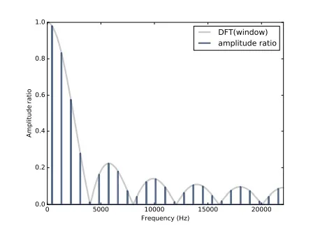
In this context, the DFT of a window is called a filter. The following figure depicts the convolution theorem.
Differenciation and Integration
Diff and Derivate
-
Diff window(operator): one-degree differentiation, like convovle with window [1, -1]
-
Derivate window:
-
Computing the difference between successive values in a signal can be expressed as convolution with a simple window. The result is an approximation of the first derivative.
-
Differentiation in the time domain corresponds to a simple filter in the frequency domain. For periodic signals, the result is the first derivative, exactly. For some non-periodic signals, it can approximate the derivative.

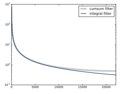
Integration
Cumsum and Integrate The cumulative sum is a good approximation of integration except at the highest frequencies, where it drops off a little faster.
Cepstrum
The cepstrum is defined as the inverse DFT of the log magnitude of the DFT of a signal
- The cepstrum calculation is different in two ways
- First, we only use magnitude information, and throw away the phase
- Second, we take the IDFT of the log-magnitude which is already very different since the log operation emphasizes the “periodicity” of the harmonics
- The cepstrum is useful because it separates source and filter
- If we are interested in the glottal excitation, we keep the high coefficients
- If we are interested in the vocal tract, we keep the low coefficients
- Truncating the cepstrum at different quefrency values allows us to preserve different amounts of spectral detail (see next slide)
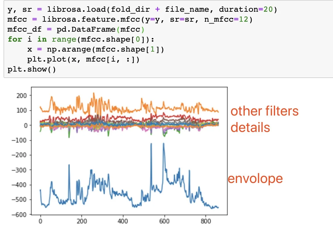
Mel Frequency Cepstral Coefficients (MFCC)