[op]drift Particle Swarm Optimization

08 Nov 2019 by BY Chih-kai Young

Particle Swarm Optimization(PSO) is a sort of classic heuristic algorithm to solve nonlinear and nonconvex optimization problem. Just like Generatic Algorith (GA), Simulated Annealing Algorithm, etc.

The PSO algorithm is known for its ease of understanding and ease of implementation. Howerver PSO also have many shortages like trapping in local optimization. Thus, many rearch about improment in PSO has implemented into more complex applications, such as Multi-stage Portfolio Optimization Problem (MSPO).

DPSO(Drift Particle Swarm Optimiation) is one of the improved PSO inpired by the motion of electrons in a conductor under electric field. Unlike PSO, DPSO is a global convergent algorithm and has strong search ability than PSO.

This article firstly introduce the classic PSO algorithm and how the DPSO improves it. Then, there is a simple test functuon for them to optimize and we can visually feel the trajectory of particle swarm motion of two algorithms.

PSO

In the PSO with $m$ particles, each particle $i$ represents a potential solution of the given problem in D-dimensional space and has three vectors at the $k^{th}$ iteration, its current position $X_{i}^{k}=\left(X_{i, 1}^{k}, X_{i 2}^{k}, \ldots, X_{i D}^{k}\right)$, its velocity $V_{i}^{k}=\left(V_{i, 1}^{k}, V_{i, 2}^{k}, \ldots, V_{i, D}^{k}\right)$ and its personal best position (the position giving the best objective function value or fitness value)$P_{i}^{k}=\left(P_{i, 1}^{k}, P_{i, 2}^{k}, \ldots, P_{i D}^{k}\right)$ There is a vector $G^{k}=\left(G_{1}^{k}, G_{2}^{k}, \ldots, G_{D}^{k}\right)$ called global best postion which is defined as the position of the best particle among all the particles in the population. The particle in PSO moves according the following equation: $V_{i j}^{k+1}=w \cdot V_{i j}^{k}+c_{1} r_{i j}^{k}\left(X_{i j}^{k}-P_{i j}^{k}\right)+c_{2} R_{i j}^{k}\left(X_{i j}^{k}-G_{j}^{k}\right)$

$X_{i j}^{k+1}=X_{i j}^{k}+V_{i j}^{k+1}$

where $c_1$ and $c_2$ are called acceleration coefficients, $w$ is the parameter which can be adjusted to the balance of exploration and exploitation, $r_{i j}^{k}, R_{i j}^{k} \sim U(0,1)$ are uniform random variables.

$P_{i}^{k}=\left\{\begin{array}{ll}{X_{i}^{k}} & {\text { if } f\left(X_{i}^{k}\right)>f\left(P_{i}^{k-1}\right)} \\ {P_{i}^{k-1}} & {\text { if } f\left(X_{i}^{k}\right) \leqslant f\left(P_{i}^{k-1}\right)}\end{array}\right.$ $G^{k}=P_{g}^{k}, \text { where } g=\arg \max _{1 \leqslant i \leqslant m}\left[f\left(P_{i}^{k}\right)\right]$

DPSO

In fact, as the particles are coverging to their own local attractors, their current position, personal best positions are all converging to one point, leading the PSO algorithm to converge. The particle’s directional movement toward $p_i^k$ is somewhat like the drift motion of an election in a con- ductor under electric field. However, besides the drift motion caused by electric field, the electron is also in thermo motion which appears to be random movement.

We change the velocity update formula as foloows: $V_{i j}^{k+1}=\alpha \cdot\left|C_{j}^{k}-X_{i j}^{k}\right| \cdot \varphi_{i, j}^{k}+c_{1} r_{i j}^{k}\left(P_{i j}^{k}-X_{i j}^{k}\right)+c_{2} r_{i j}^{k}\left(G_{j}^{k}-X_{i j}^{k}\right)$

where:

$\phi_{i,j}^k$ is a random standard normal distribution

$\sigma_{i j}^{k}=\alpha \cdot\left|C_{j}^{k}-X_{i j}^{k}\right|$ $C_{j}^{k}=(1 / m) \sum_{i=1}^{m} P_{i j}^{k}(1 \leqslant j \leqslant D)$

$\alpha$ is called compression-expansion coeffient.

and position update rule is the same as PSO: $X_{i, j}^{k+1}=X_{i, j}^{k}+V_{i, j}^{k+1}$

It can be seen that the velocity update of the DPSO compared to the PSO has nothing to do with the trajectory, and it has increased its own degree of exploration.

Test Function

Now we use a test function as follows to exam the performance of two type PSO algorithm:

It is a two dimention optimization problem and this test funtion features a lot of local optimizations.

# plot the test funtion
import matplotlib.pyplot as plt
from mpl_toolkits.mplot3d import Axes3D
import numpy as np
plt.style.use('seaborn')
fig = plt.figure()
ax = Axes3D(fig)
X = np.arange(-2, 2, 0.05)
Y = np.arange(-2, 2, 0.05)
X, Y = np.meshgrid(X, Y)
test_func = lambda X,Y: np.sin(np.sqrt(X**2+Y**2))/np.sqrt(X**2+Y**2)+np.exp((np.cos(2*np.pi*X)+np.cos(2*np.pi*Y))/2)-2.71289
Z = test_func(X, Y)
ax.plot_surface(X, Y, Z, rstride=1, cstride=1, cmap='hot')

plt.contour(X, Y, Z)

PSO (Python simple version)

N_iteration = 300
N_p = 30
px = np.random.uniform(X.min(), X.max(), size=(N_p,))
py = np.random.uniform(Y.min(), Y.max(), size=(N_p,))

c1 = 0.5
c2 = 0.01
w = 0.5
dim = 2
P = np.c_[px, py]
P_best = P
G_best = np.zeros(dim)

%matplotlib notebook
import numpy as np
import matplotlib.pyplot as plt
from matplotlib import animation
v = np.zeros((N_p, dim))
P_trace = []
fig, ax = plt.subplots()
ax.contour(X, Y, Z)
sca = ax.scatter(P[:, 0], P[:, 1], s=10, c='r')
def update(i):
    tr = P_trace[i]
    sca.set_offsets(tr)

for _ in range(N_iteration):
    func_value = test_func(P[:, 0], P[:, 1])
    global_ind = func_value.argmax()
    G_best = P[global_ind]
    for ind in range(N_p):
        r1, r2 = np.random.uniform(), np.random.uniform()
        v[ind] = w * v[ind] + c1 * r1 * (P_best[ind] - P[ind]) + \
                    c2 * r2 * (G_best - P[ind])
        P[ind] += v[ind]
        P_new_val = test_func(P[ind, 0], P[ind, 1])
        if P_new_val > func_value[ind]:
            P_best[ind] = P[ind]
    if _ % 4 == 0:
        P_trace.append(P.copy())
#     print(_, 'gloablbest', func_value[global_ind], G_best)
ani = animation.FuncAnimation(fig, update, frames=len(P_trace), interval=30, blit=True)
ani.save('pso.gif', writer='imagemagick', dpi=100)

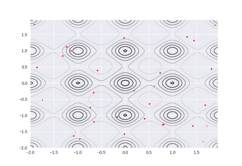
We can see the particles move more linealy to the global optimization. As long as one particle passed by globally optimal point, it will attract more particles aggregate, but on the contrary, if the number of particle is too small, it will easily fall into local optimum.

DPSO (simple python version)

N_iteration = 320
N_p = 30
px = np.random.uniform(X.min(), X.max(), size=(N_p,))
py = np.random.uniform(Y.min(), Y.max(), size=(N_p,))

c1 = 0.5
c2 = 0.01
w = 0.5
dim = 2
P = np.c_[px, py]
P_best = P
G_best = np.zeros(dim)
# dpso
v = np.zeros((N_p, dim))
P_trace = []
fig, ax = plt.subplots()
ax.contour(X, Y, Z)
sca = ax.scatter(P[:, 0], P[:, 1], s=10, c='r')
alpha = 0.09
def update(i):
    tr = P_trace[i]
    sca.set_offsets(tr)

for _ in range(N_iteration):
    func_value = test_func(P[:, 0], P[:, 1])
    global_ind = func_value.argmax()
    G_best = P[global_ind]
    C = P_best.mean(axis=0)
    for ind in range(N_p):
        r1, r2 = np.random.uniform(), np.random.uniform()
        phi = np.random.normal()
        v[ind] = alpha * np.abs(C - P[ind]) * phi + c1 * r1 * (P_best[ind] - P[ind]) + \
                    + c2 * r2 * (G_best - P[ind])
        P[ind] += v[ind]
        P_new_val = test_func(P[ind, 0], P[ind, 1])
        if P_new_val > func_value[ind]:
            P_best[ind] = P[ind]
    if _ % 4 == 0:
        P_trace.append(P.copy())
ani = animation.FuncAnimation(fig, update, frames=len(P_trace), interval=20, blit=True)
ani.save('dpso.gif', writer='imagemagick', dpi=100)

It can be seen that the particle motion of the DPSO is more random, which enhances the exploration ability and avoids falling into local optimum in the case of a small number of particles.

Next article, I will apply the DPSO algorithm into a certain problem, the multi-stage portofilo optimization problem. By repordcuting the paper our teacher suggested.

Reference

Sun J, Fang W, Wu X, et al. Solving the multi-stage portfolio optimization problem with a novel particle swarm optimization[J]. Expert Systems with Applications, 2011, 38(6): 6727-6735.
pyswarm –one python version PSO algorithm testing framework

Zhi-Kai Yang